Retina: direction selectivity, measured

Direction selectivity

A bar of light sweeps across the retina in eight directions in turn. Most cells do not care which way it moves. A minority care a great deal, and they are not a separate structure you could point to in the tissue: they sit interleaved with everything else, and the only thing that distinguishes them is what they do.

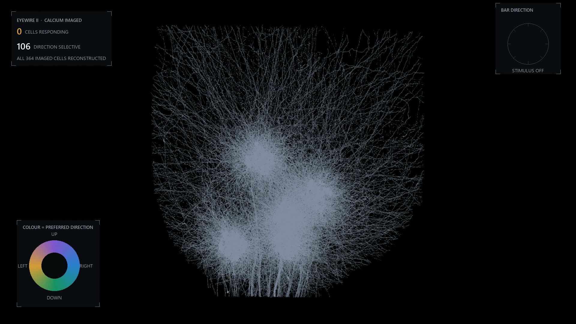
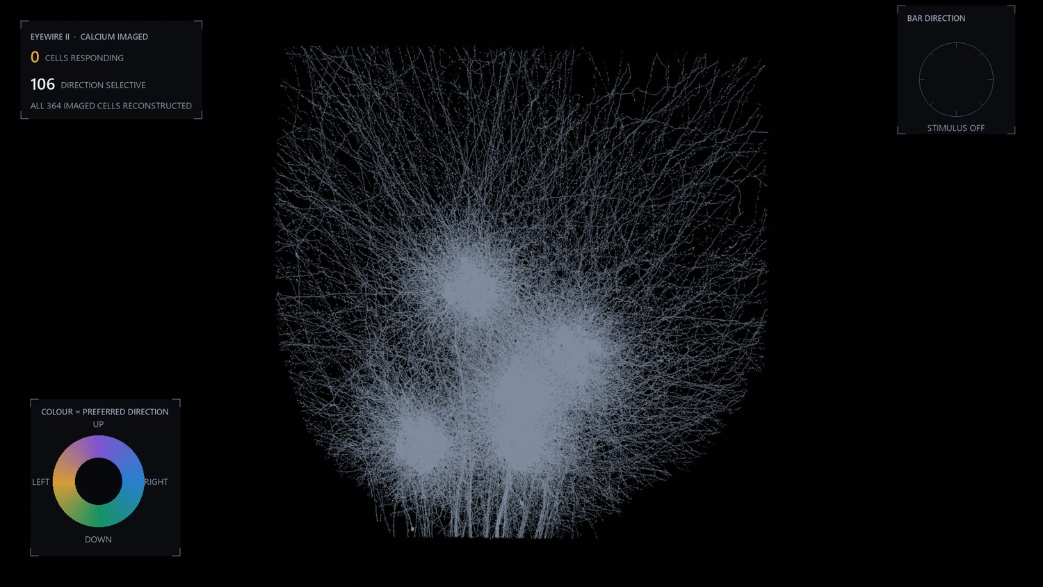
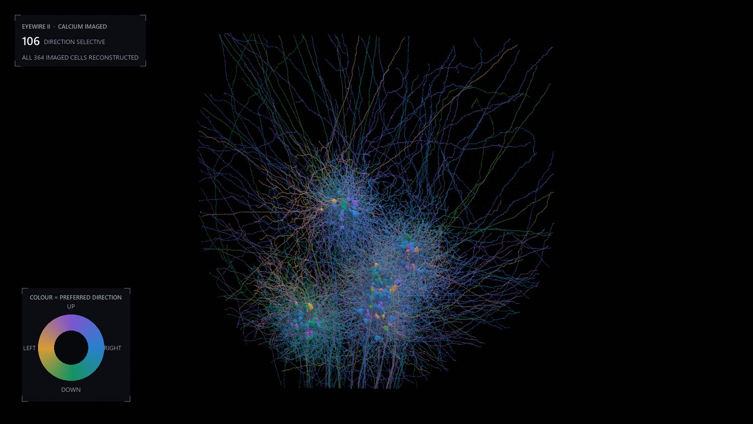
Every cell sits as a dim outline until the bar moves the way it likes. Hue is the direction it prefers and brightness is its own recorded response, so each of the 106 direction selective cells lights exactly once per sweep. The 258 that are not significantly tuned stay dim on purpose. Most of the retina is not direction selective, and hiding that would make the picture a better advertisement and a worse measurement.

prefers rightward prefers upward prefers leftward prefers downward

Colour wheels usually deserve suspicion, because they imply an order that the data does not have. This is the exception. Preferred direction is an angle, so it needs a map that wraps, where the value just below 360 degrees sits next to the value just above zero. The four colours are the CA3 house palette spaced evenly around the circle, so the map still wraps and still means an angle without becoming a rainbow.

The four stages

The film moves through four pictures of the same 364 cells, and each one answers a different question. They are worth seeing still, because a legend is hard to read while the thing underneath it is moving.

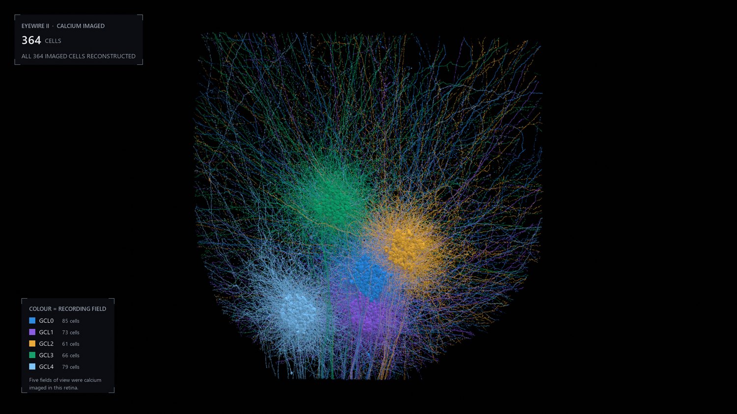
All 364 reconstructed retinal cells in plain grey, no colour applied — **The reconstruction.** Every cell with both a calcium recording and a mesh, with no measurement painted on it yet. This is the structure the rest is drawn onto.

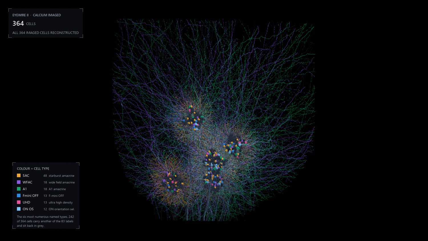
The same cells coloured by which of five recording fields they came from, appearing as five separate clusters — **Colour is the recording field.** Five separate two photon fields, GCL0 to GCL4. They sit apart because the microscope looked at five patches, not because the retina is organised that way. This is the one stage where the colour is about the experiment rather than the tissue.

The same cells recoloured by anatomical cell type — **Colour is cell type.** 83 named types across 364 cells, 213 ganglion and 151 amacrine. Seventy of them carry no type at all, and those stay grey rather than being given a plausible one.

Only the direction selective cells remain lit, coloured by preferred direction — **Everything not direction selective falls away.** 106 cells survive, coloured by the direction each one prefers. They are scattered through the sheet rather than gathered, which is the point: you could not find them by looking at the anatomy.

How the direction gets computed

Direction selectivity is not made in the brain. It is already finished by the time the signal leaves the eye, and the cell most responsible is the starburst amacrine cell. Its dendrites radiate from the cell body like a firework, and the direction computation happens along those individual branches.

The 24 shown below are a sample, not the population. There are 48 starburst cells in the calcium imaged set and the reconstruction holds several hundred more, so this film is a sample twice over. It shows 24 because that is how many had a usable mesh when it was made; the rebuilt library now covers all 48, and this film has not been remade to match. That matters for what this film can and cannot be used to claim: the real sheet is far denser than what you are about to watch, and any impression you get here about how much neighbouring starburst cells overlap is an artefact of my sampling rather than a fact about retina. What survives the sampling is the depth, because where a cell puts its dendrites does not depend on which other cells I happened to include.

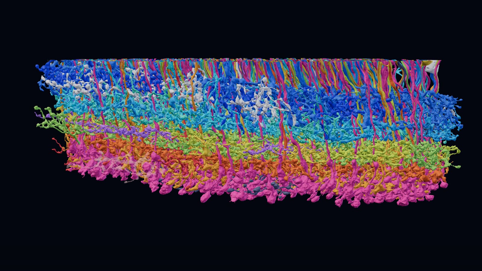
The 24 sampled starburst amacrine cells are laid in one at a time, each in its own colour, so you can see the individual arbors before they pile up. Then the whole thing turns on its side. Every arbor collapses into one thin band, with the cell bodies sitting above it on short stalks. That flatness is the point: two cells can only form a synapse where both of them are, so committing to a depth is most of what wiring a retina means. It is also the claim here that a partial sample cannot break, since adding the missing cells can only make the band more crowded, not move it.

The turn is a real rotation of the reconstruction, not a second render from a second angle, and the sag you can see across the band is real too. This tissue was not cut perfectly parallel to its own layers. I have not flattened it, because the flattening would be the only fictional thing in the frame.

What is measured and what is not

Element	Where it comes from
Cell shape	Electron microscope reconstruction, EyeWire II
Hue in the first film	Recorded preferred direction of the cell
Brightness in the first film	The cell's own calcium response at that bar direction
Which cells count as tuned	Permutation test on the recording, p < 0.05
Depth of the starburst band	Geometry of the reconstruction
Colour of each starburst cell	Chosen, and means nothing but identity
Speed of everything	Chosen, so it can be watched

The bar itself is not drawn. Two attempts put a bright slab across the mosaic and both hid the cells they were meant to explain, so the sweep is carried by the cells lighting in sequence instead, each following its own measured tuning curve. The direction being swept is shown on the compass in the corner.

Joining two experiments

The hard part of this was not rendering. It was deciding which reconstructed cell is which recorded cell, and the obvious routes both failed. Matching on segment identifiers returned nothing, because those identifiers are versioned and get rewritten every time somebody proofreads a merge. Matching on supervoxels did better and still recovered only a small fraction.

What worked was the crudest option: cell body coordinates. A soma is a large object in a fixed place, and both experiments recorded where they are. That match is the reason there is anything on this page.

Everything on this page is drawn from that intersection, which is much smaller than either experiment. The reconstruction contains far more cells than were imaged, and the recordings cover cells that have not been reconstructed. Any count below is a count of the overlap, and should never be read as a count of the dataset.

364

cells rendered

named cell types

213 / 151

ganglion / amacrine

0.21 to 0.70

direction selectivity index

Ten thousand bipolar cells

Bipolar cells are the retina's relay. They carry the signal from the photoreceptors to the ganglion cells that send it to the brain, and on the way they split it into more than a dozen parallel channels, one for each type. In October 2026 the citizen scientists of EyeWire II finished proofreading their 10,000th bipolar cell in this reconstruction, every one checked branch by branch by hand.

The film and the model below show 981 of them: every proofread bipolar cell whose cell body sits within about 80 micrometres of one point in the volume, roughly a tenth of the total. Nineteen cells nearer that point are left out, because their recorded position or their branches put them well outside the patch. The types are a classifier's predictions, not labels anyone drew by hand.

The cells arrive in the order they were proofread, coloured by type. Turned on their side they sort into bands, because each type sends its axon terminals to its own depth of the inner retina, where it meets the cells it passes its signal to. Then each cell takes the colour of the citizen scientist who proofread it.

The same 981 bipolar cells seen from the side, coloured by type — The same 981 cells, live. **Drag to turn them, scroll or pinch to zoom,** and point at a cell to see its type and who proofread it. Click a name in the key to hide or show those cells. Open it full screen to play the whole film live, with the cells still yours to turn whenever you pause.

Unlike the two films above, the bipolar film was not rendered in Blender. It is a web page: the meshes come straight from the segmentation through CAVE, are drawn with three.js, and a browser with no screen captured it one frame at a time. The model above is that page with the controls left on, each cell simplified to about two thousand triangles so the whole patch loads in one go.

Sources

Reconstruction and cell type labels: the stroeh_mouse_retina dataset on eyewire.ai, served through CAVE. Light responses and direction tuning: the Euler lab's calcium imaging of the same tissue, via eyewire2-functional-analysis. The direction selectivity and starburst films were rendered in Blender with EEVEE Next. Bipolar cell proofreading: the citizen scientists of EyeWire II, with types from the project's classifier; the bipolar film and model are drawn in the browser with three.js.